Quickstart with Deeplearning4J
Deep learning, i.e. the use of deep, multi-layer neural networks, is the major driver of the current machine learning boom. From great leaps in quality in automatic translation, over autonomous driving, to beating grandmasters in the game Go, this technique has made a lot of headlines.
Deeplearning4J, also called DL4J, is a Java library for Deep Learning. But, it also a whole family of other libraries that simplify the use of deep learning models with Java. As an alternative to the many Python based frameworks, DL4J offers a way to easily bring Deep Learning into existing enterprise environments.
This blog post shows how to get started with DL4J in no time. By using an example where the goal is to predict whether a customer will leave his bank, each step of a typical workflow is considered. In order to focus on the individual steps, only excerpts of the code currently being discussed are shown. Imports and other Java boilerplate are left out, but the complete code including training data can be found at https://github.com/treo/quickstart-with-dl4j.
Update 30.11.2020: Finally came around to updating this to use version 1.0.0-beta7. Changed a few hyper parameters due to the way regularization handling changed; Updated companion project with the fixes necessary to run on Java 15; Updated links to community forum.
Update 20.02.2019: Finally came around to updating this to use version 1.0.0-beta3. Changed a few hyper parameters; Added some additional headings for the DataVec section; Updated companion project with the fixes necessary to run on Java 11.
Update 07.11.2018: Version 1.0.0-beta3 has been released. I’ll update this post shortly. The model shown here needs to be retuned and the dependency declaration for ParallelInference needs to be updated. In the meantime check out the release notes for Deeplearning4J 1.0.0-beta3.
- Integrating DL4J into your project
- Loading data
- Training the model
- Using the Model
- Beyond the quickstart
- Closing remarks
Integrating DL4J into your project
DL4J, like many other Java libraries, can easily be included as yet another dependency in the build tool of choice. In this post, the necessary information is given in Maven format, as it would be seen in a pom.xml file. Of course, you can also use another build tool like Gradle or SBT.
DL4J is not intended to be used without build tools, since it itself has a large number of direct and transitive dependencies. Therefore, there is no single jar file that you could manually specify as a dependency in your IDE. DL4J and its libraries have a modular structure so that you can adapt its dependencies to the needs of your project. Especially for beginners this can make getting started a bit more complicated, because it is not necessarily obvious which submodule is needed to make a certain class available.
The used versions of all DL4J modules should always be the same. To simplify version management, we define a property which we will use in the following to specify the version. DL4J is currently close to its 1.0 release and in this post, we are using version 1.0.0-beta7, which has only recently been released.
<properties>
    <dl4j.version>1.0.0-beta7</dl4j.version>
</properties>
For the beginner it is advisable to start with the deeplearning4j-core module. It includes many other modules transitively and thus allows the use of a multitude of features without having to search for the right dependency. The disadvantage is that when bundling all dependencies into an Uberjar you will get a large file.
<dependency>
    <groupId>org.deeplearning4j</groupId>
    <artifactId>deeplearning4j-core</artifactId>
    <version>${dl4j.version}</version>
</dependency>
DL4J supports multiple backends, which allows the use of CPU or GPU. In the simplest case, the backend is selected by specifying a dependency. To use the CPU backend, nd4j-native-platform is required. For the GPU backend, nd4j-cuda-X.Y-platform is used, where X.Y should be replaced by the installed CUDA version. Currently CUDA 10.0, 10.1 and 10.2 are supported.
 <dependency>
    <groupId>org.nd4j</groupId>
    <artifactId>nd4j-native-platform</artifactId>
    <version>${dl4j.version}</version>
</dependency>
Both backends rely on the use of native binaries, which is why the platform modules also include the binaries for all supported platforms. This allows distributing an Uberjar to several different platforms without having to create a single specialized jar file for each one of them. The currently supported platforms for the CPU backend are: Linux (PPC64LE, x86_64), Windows (x86_64), macOS (x86_64), Android (ARM, ARM64, x86, x86_64); for CUDA-enabled GPUs: Linux (PPC64LE, x86_64), macOS (x86_64), Windows (x86_64).
As the last dependency for a basic setup, we add a logger. DL4J requires an SLF4J-API compatible logger to share its information with us. In this example we use Logback Classic.
<dependency>
    <groupId>ch.qos.logback</groupId>
    <artifactId>logback-classic</artifactId>
    <version>${logback.version}</version>
</dependency>
As can already be seen from the specification of the backend, ND4J forms the foundation on which DL4J builds. ND4J is a library for fast tensor math with Java. In order to make maximum use of the available hardware, practically all calculations are carried out outside the JVM. This way CPU features such as AVX vector instructions and GPUs can be utilized.
If a GPU is used, however, it should be known that for deep learning in particular, a quite potent GPU is often required to achieve a speed advantage over a CPU. This is especially true for notebook GPUs that were released before the current GeForce 1000 series, and even on the desktop you should at least have a GeForce GTX 960 with 4GB RAM. The reason for this recommendation is that GPUs shine especially with calculations on large amounts of data - but these large amounts of data also require a corresponding amount of RAM and this is only available in sufficient quantities with the more powerful models.
Loading data
As with all other forms of Machine learning, in order to do any deep learning, data has to be collected and loaded first. This blog post focuses on tabular data available as CSV files. However, the procedure for other file formats, or other data types such as images, is similar.
Basically, if you want to get good results quickly, you should have a good understanding of your data and the problem to be solved. Some expert knowledge about the data and the general problem area, as well as an appropriate preparation of the data, can significantly reduce the model complexity and training time in many cases.
Another point to note is that you have to divide your data into at least two parts to train a model. Most of the data, usually about 80%, is used for training and is therefore referred to as the training set. The remaining data, usually around 20%, is used to evaluate the quality of the model and is referred to as the test set. Especially when more advanced tuning is required, it is also common to reserve another 10% of the training data for a validation set to check whether the model has been overfitted to the test set.
When selecting data for the test set, it should be noted that it should consist of a representative subset of all data. This is necessary to be able to check the informative value of the model properly. The same is true for the validation set in cases where it is used.
The data set used in this blog post comes from Kaggle, a platform for data science and machine learning competitions. It consists of tabular data and contains not only purely numerical but also categorical data. It has already been preprocessed somewhat and split into a training set and a test set.
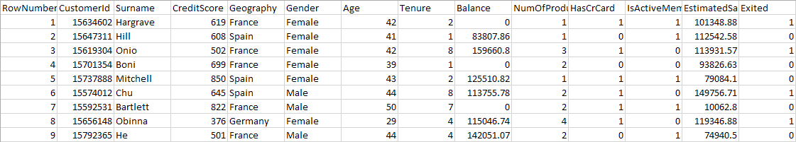
The data set consists of a bank’s customer data. Each line represents a customer and, in the column “Exited” also contains the information whether the customer has left the bank. The problem we want to solve in this example is to train a model that can use this customer data to predict whether a customer will leave the bank. So, it is a classic classification problem with 2 classes: “Will remain customer” and “Will leave the bank”.
DataVec
Like all other statistical machine learning methods, deep learning only works with numerical data. DataVec is a DL4J library that supports us in loading, analyzing and converting our data into the necessary format. To use it, we do not need to specify another dependency, since it is already loaded as a transitive dependency of the deeplearning4j-core module.
In this example we will encounter the three core concepts of DataVec. These consist of the InputSplit, RecordReader and TransformProccess. They can be understood as the steps that the data must go through in order to be enriched from raw data to actually usable data.
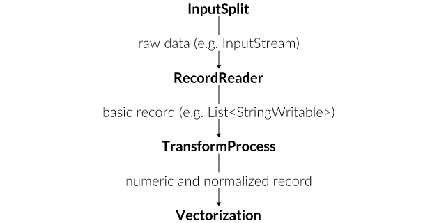
We start by creating a FileSplit. The task of the InputSplit will be to provide the RecordReader with a single input. We pass it the folder where our training set is located as a File instance, and an optional Random object. By providing that random object, FileSplit will read the files in a random order. This will become important later for training.
Random random = new Random();
random.setSeed(0xC0FFEE);
FileSplit inputSplit = new FileSplit(new File("X:/Churn_Modelling/Train/"), random);
In addition to FileSplit, there are a number of other implementations of InputSplit that can provide data from an Input Stream or a Collection, for example.
Our data is CSV formatted, therefore we create a CSVRecordReader and initialize it with the previously created InputSplit. The RecordReader will then take the input it receives from the InputSplit and divide it into one or more examples. These examples can then be retrieved from the RecordReader in the form of records.
CSVRecordReader recordReader = new CSVRecordReader();
recordReader.initialize(inputSplit);
As with the FileSplit, DataVec also provides different implementations for the RecordReader interface, like readers for Excel files, pictures, videos or even (via JDBC connected) databases.
Defining a Schema
Records are basically nothing more than lists of values. And especially in the case of the CSVRecordReader, these values are all strings. In order to continue working with them, we have to define a schema for our data. Similar to the schema you may know from SQL databases, we specify here which types of values can be in a record. Due to the fact that a record is a list of values, we also have to pay attention to the order of the column definitions here, since it must correspond to the order in our CSV files.
Schema schema = new Schema.Builder()
                .addColumnsInteger("Row Number", "Customer Id")
                .addColumnString("Surname")
                .addColumnInteger("Credit Score")
                .addColumnCategorical("Geography", "France", "Germany", "Spain")
                .addColumnCategorical("Gender", "Female", "Male")
                .addColumnsInteger("Age", "Tenure")
                .addColumnDouble("Balance")
                .addColumnInteger("Num Of Products")
                .addColumnCategorical("Has Credit Card", "0", "1")
                .addColumnCategorical("Is Active Member", "0", "1")
                .addColumnDouble("Estimated Salary")
                .addColumnCategorical("Exited", "0", "1")
                .build();
Here it is already worthwhile to know your data at least superficially. For example, we have already specified all possible values for the “Geography” and “Gender” columns in the schema, and we have specified the numbers 0 and 1 for “Has Credit Card”, “Is Active Member” and “Exited” as categorical instead of declaring them as integers. This is because experience has shown that such yes/no information works better as categorical data (with one-hot encoding, see below).
Analyzing the data
In the next step, we will first have the data analyzed. For this we use a new feature, called AnalyzeLocal, which is not made available by the deeplearning4j-core module and therefore requires us to add another dependency. Due to an incompatibility of datavec-arrow with the UI Server we are going to use later, we need to exclude it from being transitively included.
 <dependency>
    <groupId>org.datavec</groupId>
    <artifactId>datavec-local</artifactId>
    <version>${dl4j.version}</version>
    <exclusions>
        <exclusion>
            <groupId>org.datavec</groupId>
            <artifactId>datavec-arrow</artifactId>
        </exclusion>
    </exclusions>
</dependency>
After adding the dependency, running the analysis is easy. We specify the Schema and RecordReader as parameters and get a result.
DataAnalysis analysis = AnalyzeLocal.analyze(schema, recordReader);
HtmlAnalysis.createHtmlAnalysisFile(analysis, new File("X:/Churn_Modelling/analysis.html"));
We can also output the result in human-readable form as an HTML file. With the help of the analysis output, we can get even more familiar with the data. For each column we get an evaluation of how its values are distributed and a histogram as a visualization of this distribution.
We pay particular attention to the value range of the numeric columns. For the training of neural networks, it is recommended that each input lies in a range between -1 and 1, otherwise you quickly leave the functional range of activation functions and regularization methods - the effect is that the model does not learn.
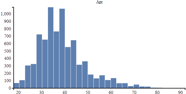
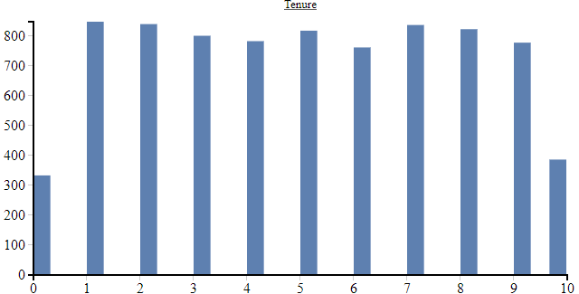
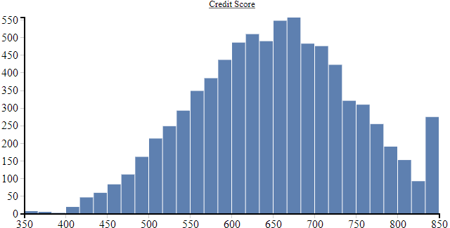
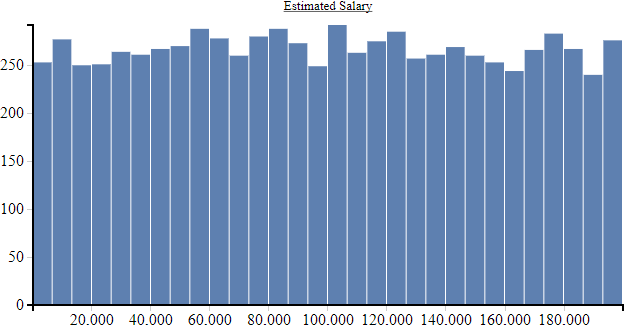
We see that in many cases the value range lies outside the recommended -1 to 1 range. So, we will have to normalize this data before we can continue using it. However, in addition to normalization, there is also further preparatory work to be done.
Transformation and Normalization
Here we come to the last step before we can vectorize the data: the TransformProcess. We use it to implement what we have learned from the analysis. We start by removing the columns “Row Number”, “Customer Id” and “Surname”, as these seem useless for the problem and could lead to training problems down the road.
The columns, which we have classified as categorical right from the start, are now transformed into a one-hot encoding. This means that each category gets its own column. Each, but one, of those columns is set to 0. The one column that gets a 1 is exactly the column of the corresponding category. This type of encoding is always useful when you have data that does not have a natural translation into a numerical form and cannot be sorted. In our example it would make no sense to code the countries of the “Geography” column as 0,1,2, since each country could assume any of these values. Instead, the “Geography” column becomes 3 different columns that can be interpreted as “Is in [country]”.
This transformation can also be applied to columns with integer values, which happens in the example for the “Num Of Products” column. Although this information is numerical, some intuition about the data helps here. We use a one-hot encoding for this column, because, when it comes to determining if the customer is going to stay or leave his bank, a customer who uses more of the bank’s products is probably different in nature from a customer who only uses one of the bank’s products.
TransformProcess transformProcess = new TransformProcess.Builder(schema)
                .removeColumns("Row Number", "Customer Id", "Surname")
                .categoricalToOneHot("Geography", "Gender", "Has Credit Card", "Is Active Member")
                .integerToOneHot("Num Of Products", 1, 4)
                .normalize("Tenure", Normalize.MinMax, analysis)
                .normalize("Age", Normalize.Standardize, analysis)
                .normalize("Credit Score", Normalize.Log2Mean, analysis)
                .normalize("Balance", Normalize.Log2MeanExcludingMin, analysis)
                .normalize("Estimated Salary", Normalize.Log2MeanExcludingMin, analysis)
                .build();

Schema finalSchema = transformProcess.getFinalSchema();
In choosing the appropriate normalization for the remaining columns, we are guided by the results of the analysis. As a rule of thumb, a MinMax normalization can be used for equally distributed values; a Standardize normalization is used for normally distributed values; and logarithmic normalization is often appropriate for values covering a wide range. This rule of thumb gives us the initial step, but in practice you should also consider other normalizations and see if they might work better for your problem. In this example, we are using a logarithmic normalization for the “Credit Score” value, although the data in the analysis shows the typical bell shape of a normal distribution.
Most normalization methods require statistical information about the data set to function. Here, too, the analysis we made earlier helps us. Since the analysis also knows the original schema, the TransferProcess can access the statistical information directly with the specified column name.
Vectorization
The next step is to vectorize the data. Usually Deep Learning does not consider all training data at every training step, but only a fraction of it. This process is called mini-batching. Every full run through the data is called an epoch. We’d like that for each epoch, the mini-batches consist of different examples, since that helps in training a better model. For this reason, we instantiated the InputSplit at the beginning together with a Random object.
The size of the mini-batch, the so-called batch size, determines how many examples the model sees during each training step and thus also significantly influences the training regime. A larger batch size results in fewer mini-batches and thus fewer training steps in each epoch. At the same time, however, the model gets to see more data and may be able to find better patterns.
int batchSize = 80;
We set the value for our case to 80, since we have 8000 examples in the training set and this leads to a clean cut of 100 mini-batches.
Using the just defined TransformProcess we create a new RecordReader, which will first read in the CSV data and then transform it immediately. As before, we initialize the record reader with the InputSplit that refers to our training data.
TransformProcessRecordReader trainRecordReader = new TransformProcessRecordReader(new CSVRecordReader(), transformProcess);
trainRecordReader.initialize(inputSplit);
Then a DataSetIterator is created, which reads the transformed data from the RecordReader, vectorizes it and takes care of building mini-batches. Since we want to solve a classification problem, we use the classification method to indicate in which column our label, i.e. the target value, can be found and how many possible classes there are. We will use this DataSetIterator to train our model.
RecordReaderDataSetIterator trainIterator = new RecordReaderDataSetIterator.Builder(trainRecordReader, batchSize)
                .classification(finalSchema.getIndexOfColumn("Exited"), 2)
                .build();
If you do not want to use DataVec, you can also implement the DataSetIterator interface yourself. However, this is usually only necessary if you have special needs for the pre-processing of your data or have special requirements when creating mini-batches.
Training the model
Before we can start training a model, we must first define what the model should look like. In contrast to many other machine learning methods, Deep Learning has a lot more options that have to be considered. You have to decide which architecture the network should use, how wide the individual layers should be, and which values many other hyperparameters should take. If you are lucky, there is a pre-trained model that can solve your own problem. Or maybe there is at least a paper describing a network architecture which you can use to orientate yourself.
Defining the structure
Basically, the network design depends on the specific problem you are dealing with. Convolutional layers are always useful where spatial contexts are interesting, e.g. in pictures. Recurrent layers are useful when sequences of data are to be processed and the order within the sequence is important. And Dense layers, also known as fully connected layers, are good if all existing data is to be considered at once.
Finding a good network architecture is a task that relies on experimentation. You have to try many ideas and conduct many experiments to find a really good model. As a guideline you can use the rule of thumb that you should start with simple models, i.e. models with few, narrow layers, and add complexity only slowly. If you can’t overfit your model, i.e. reduce the error to 0, on a fraction of your data, like a single mini-batch, then the model will probably not be able to learn anything, even if you give it more data.
For our example we will use a simple multi-layer model. First, we set a random seed, since model weights will be initialized randomly – in our case using the XAVIER initialization scheme. Setting a random seed is always recommended, especially if you have not yet fixed a model and its hyperparameters, as otherwise good results could simply happen by chance and these would no longer be reproducible. Next, the TANH activation function is set as a default for each layer. This is a practical shortcut, that allows us to avoid setting it on each layer individually. The updater used here is Adam with a learning rate of 0.001 and a L2 regularization of 0.0000316.
 MultiLayerConfiguration config = new NeuralNetConfiguration.Builder()
                .seed(0xC0FFEE)
                .weightInit(WeightInit.XAVIER)
                .activation(Activation.TANH)
                .updater(new Adam.Builder().learningRate(0.001).build())
                .l2(0.000316)
                .list(
                        new DenseLayer.Builder().nOut(25).build(),
                        new DenseLayer.Builder().nOut(25).build(),
                        new DenseLayer.Builder().nOut(25).build(),
                        new DenseLayer.Builder().nOut(25).build(),
                        new DenseLayer.Builder().nOut(25).build(),
                        new OutputLayer.Builder(new LossMCXENT()).nOut(2).activation(Activation.SOFTMAX).build()
                )
                .setInputType(InputType.feedForward(finalSchema.numColumns() - 1))
                .build();
In this case, the model architecture consists of 5 DenseLayers each with 25 output units and one OutputLayer with 2 outputs. An OutputLayer itself is in principle also a DenseLayer, but the difference is in the loss function, which is also specified there. It calculates the deviation between what the model outputs during training and the label. With this deviation, the model is then adjusted to provide better results. The OutputLayer also sets a different activation function from the default TANH and uses a SOFTMAX activation instead. This ensures that the output of the model can be interpreted as a probability distribution, i.e. that each value is between 0 and 1 and the sum of all values is exactly 1.
Finally, setInputType is used to set what type of data the model will process (feedForward) and how many input columns the examples have. This will then automatically calculate the number of inputs for each layer, so we don’t have to specify it manually. For more complex models, this also adds the necessary adapters between two layer types automatically where needed.
All parameter values selected here are the result of some trial and error. For example, the TANH activation function has proven to be more effective for this problem than the now more commonly used RELU activation function.
Training
The actual training is pretty simple compared with the effort that it takes to come up with a good model architecture. We first create a new model from the previously defined configuration, initialize it and then train it using the training set for 60 epochs, i.e. the training set is iterated over 60 times during the training. After some time, the training finishes and the trained model can be used.
MultiLayerNetwork model = new MultiLayerNetwork(config);
model.init();
model.fit(trainIterator, 60);
The actual training always revolves around calling the fit method. DL4J has several variants to offer. The variant used in the example above accepts a DataSetIterator and an epoch number. If the epoch number is omitted, data is iterated over exactly once, i.e. the model is trained for one epoch. The last variant is that you iterate through the iterator yourself, and therefore also pass the next mini-batch to the fit method yourself.
Which of the different training methods you should use depends on what you want to do with the model between training sessions. For example, one could evaluate the model between each epoch, store different training states or manipulate the model in any other way.
Evaluation
After the model has been trained, one also wants to evaluate how well it generalizes on data it has not yet seen. The test set is used for this purpose. To use the test set, we load it the same way as we did for the training set. In this case, the batch size is irrelevant for the result, so for simplicity’s sake we will use the same one as for the training set.
TransformProcessRecordReader testRecordReader = new TransformProcessRecordReader(new CSVRecordReader(), transformProcess);
testRecordReader.initialize( new FileSplit(new File("X:/Churn_Modelling/Test/")));
RecordReaderDataSetIterator testIterator = new RecordReaderDataSetIterator.Builder(testRecordReader, batchSize)
        .classification(finalSchema.getIndexOfColumn("Exited"), 2)
        .build();
DL4J makes the evaluation of a model easy: it is usually sufficient to call the evaluate method on the model together with the test set. You get an Evaluation object, which is most often used to just display the evaluation summary somewhere. In our example, we write the summary to the console.
Evaluation evaluate = model.evaluate(testIterator);
System.out.println(evaluate.stats());
========================Evaluation Metrics========================
 # of classes:    2
 Accuracy:        0,8710
 Precision:       0,7208
 Recall:          0,5093
 F1 Score:        0,5969
Precision, recall & F1: reported for positive class (class 1 - "1") only


=========================Confusion Matrix=========================
    0    1
-----------
 1551   74 | 0 = 0
  184  191 | 1 = 1

Confusion matrix format: Actual (rowClass) predicted as (columnClass) N times
==================================================================
But, the evaluation object can also be used to access other evaluation metrics that where not shown in the summary by default. In our case, the Matthews correlation coefficient is particularly noteworthy, as it also considers the unequal distribution within the data, and thus shows that despite good accuracy, the predictive strength of this model is still somewhat limited.
System.out.println("MCC: "+evaluate.matthewsCorrelation(EvaluationAveraging.Macro));
MCC: 0.5339438422006081
Tuning
Since training can take a long time, especially if you have a lot of data, you often don’t want to blindly belive that it will go well. This is especially important if you have not yet selected the optimal hyperparameters.
Hyperparameters are all parameters that define the exact form of the model and the training regime. There are two types of parameters: the parameters learned by the model, also called weights, and the hyperparameters specified by the user. Hyperparameters include, among others, the learning rate, the strength of regularization, the size of a mini-batch and also the size and number of layers in the network. Choosing good hyperparameter is still more art than science at the moment, but there are tools to help us.
First, we look at listeners which help by providing additional information during the training. In general, listeners are added to a model using the addListeners method. In the example two different listeners will be used. The ScoreIterationListener can be used without adding further dependencies and simply logs the training score, i.e. the value of the loss function on the current mini-batch. It is thus parameterized only with how often it should make an output. In our example, this happens every 50 iterations, i.e. after 50 mini-batches or twice per epoch.
model.addListeners(new ScoreIterationListener(50));
Since it outputs the value of the loss function at the given iteration, we want that value to be decreasing.
[main] INFO org.deeplearning4j.optimize.listeners.ScoreIterationListener - Score at iteration 0 is 0.6176512682074273
[main] INFO org.deeplearning4j.optimize.listeners.ScoreIterationListener - Score at iteration 50 is 0.417752781122097
[main] INFO org.deeplearning4j.optimize.listeners.ScoreIterationListener - Score at iteration 100 is 0.3902740254303334
The StatsListener is much more complex and is used together with a web interface. In order to use it another dependency is needed.
 <dependency>
    <groupId>org.deeplearning4j</groupId>
    <artifactId>deeplearning4j-ui</artifactId>
    <version>${dl4j.version}</version>
</dependency>
If the StatsListener is used as shown in the example, you get a hint in the log where the web interface can be found. Per default it can be found at http://127.0.0.1:9000. Like the ScoreIterationListener, it can also be parametrized to collect information only in certain intervals. In this example, we are again going with 50 iterations, or twice per epoch.
UIServer uiServer = UIServer.getInstance();
StatsStorage statsStorage = new InMemoryStatsStorage();
uiServer.attach(statsStorage);
model.addListeners(new StatsListener(statsStorage, 50));

model.fit(trainIterator, 60);
The web interface shows a lot of information that can be used to see whether the training is progressing well. A score-graph that tends to fall is particularly important. If it rises, the behavior is called divergent, i.e. the model does not only learn nothing, it becomes increasingly worse. In the screenshot you can see that the score for each mini-batch fluctuates, but still decreases on average, so you should not assume a divergence on the first ascent, but only when there is actually a continuing upward trend.
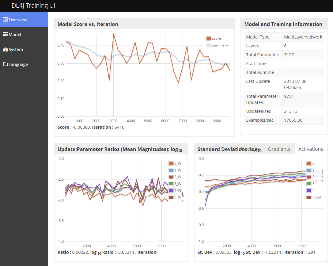
Another important information shown here is the Update to Parameter Ratio. The rule of thumb is that you should aim for a value around -3.0. This can be done by changing the learning rate. If the value is too high, e.g. -1.0, the learning rate should be reduced and if it is too low, e.g. -4.0, the learning rate should be increased.
As useful as the listeners are, you should also remember that they affect performance. If you want to train a model completely unattended, you should not slow down the process unnecessarily by collecting information that is never made visible.
Trying to manually figure out which hyperparameters provide the best training progress and the best result can quickly consume a lot of time. That’s where the next tool comes in: the Arbiter library from DL4J supports an automated search for good hyperparameter combinations. For the advanced user it is definitely worth a look.
Pro tip: When manually looking for a good L2 regularization value, start out with an order of magnitude value close to $\sqrt \frac{batchSize}{TotalExampleCount \times Epochs}$ , in this example using 100 epochs, this is $0.01 = 10^{-2}$ and start reducing it by orders of magnitude, i.e. go from $10^{-2}$ to $10^{-3}$ to $10^{-4}$ and so on. Once you find something that works, try bisecting the order of magnitude, i.e. go from $10^{-3}$ to $10^{-3.5}$ (= 0.000316…). This is how the value in this example was found.
Saving
Saving the model is also quite simple. By calling the saveFile method, the model is written to the specified file. By default, the Updater state is also saved. This is necessary if you want to continue training the saved model later. If you want to omit the Updater state, you can pass false as the second parameter to saveFile.
File modelSave = new File("X:/Churn_Modelling/model.bin");
model.save(modelSave);
Usually, however, not only the model must be saved. If normalizations have been applied which depend on statistical information, then it is also necessary to save this information for future use, since you will also have to apply the exactly same normalizations on new data. You can add any other data into the model file. Note, however, that this will use Java’s serialization function. It is therefore appropriate to convert your data into the simplest possible format, before passing it to the addObjectToFile method, in order to have data that will still be loadable with newer versions.
In the example we save not only the model, but also the result of the analysis and the schema of the model input data.
ModelSerializer.addObjectToFile(modelSave, "dataanalysis", analysis.toJson());
ModelSerializer.addObjectToFile(modelSave, "schema", finalSchema.toJson());
Using the Model
Loading the model is as easy as saving it. We specify the file from which the data should be loaded and load the model and any additionally stored data.
File modelSave = new File("X:/Churn_Modelling/model.bin");
MultiLayerNetwork model = ModelSerializer.restoreMultiLayerNetwork(modelSave);
DataAnalysis analysis = DataAnalysis.fromJson(ModelSerializer.getObjectFromFile(modelSave, "dataanalysis"));
Schema targetSchema = Schema.fromJson(ModelSerializer.getObjectFromFile(modelSave, "schema"));
We assume that the data will come from a different source than the training data. So, we will not be able to reuse our CSVRecordReader. For this example, we are even going one step further and skip a record reader at all. Rather we will hard code it for the example, but putting a DTO with its getters in place would be just as easy.
List rawData = Arrays.asList(26, 8, 1, 547, 97460.1, 43093.67, "France", "Male", "1", "1");
As with training, we start by defining a scheme and a TransformProcess. The big difference to training is that this time, we get the data in a different order and the unnecessary data does not even appear in the schema.
Schema schema = new Schema.Builder()
                .addColumnsInteger("Age", "Tenure", "Num Of Products", "Credit Score")
                .addColumnsDouble("Balance", "Estimated Salary")
                .addColumnCategorical("Geography", "France", "Germany", "Spain")
                .addColumnCategorical("Gender", "Female", "Male")
                .addColumnCategorical("Has Credit Card", "0", "1")
                .addColumnCategorical("Is Active Member", "0", "1")
                .build();
As a result, the TransformProcess has also to be somewhat different. This time there is no need to remove data, but it is necessary to put the columns back in the order they were used during the training, otherwise the model will not be able to use the data.
String[] newOrder = targetSchema.getColumnNames().stream().filter(it -> !it.equals("Exited")).toArray(String[]::new);
That is the reason why we also saved the schema of our model input data. That way we can use it to reorder the new columns by name, rather then ensuring that they are provided in the correct order when converting the data into a record. To reorder the columns into the same order as was used in training, we use the stored schema, in which we remove the “Exited” column, since that is what we want to predict in production and is therefore not contained in our data any more.
Since the TransformProcess is still responsible for normalization, it also needs the previously saved analysis.
TransformProcess transformProcess = new TransformProcess.Builder(schema)
                .categoricalToOneHot("Geography", "Gender", "Has Credit Card", "Is Active Member")
                .integerToOneHot("Num Of Products", 1, 4)
                .normalize("Tenure", Normalize.MinMax, analysis)
                .normalize("Age", Normalize.Standardize, analysis)
                .normalize("Credit Score", Normalize.Log2Mean, analysis)
                .normalize("Balance", Normalize.Log2MeanExcludingMin, analysis)
                .normalize("Estimated Salary", Normalize.Log2MeanExcludingMin, analysis)
                .reorderColumns(newOrder)
                .build();
Now we convert our data into a record, transform it and vectorize the result to a format that is accepted by the model. Since we are using only a single record, it is practically a mini-batch of size 1.
List<Writable> record = RecordConverter.toRecord(schema, rawData);
List<Writable> transformed = transformProcess.execute(record);
INDArray data = RecordConverter.toArray(transformed);
As we want to perform a classification with our model, and its output is assigned a Softmax activation function, we can query the model with the predict method and get an integer array of answers.
int[] labelIndices = model.predict(data); // = [0] = Will stay a customer
We get an array, instead of just a single answer, because the model always assumes a batch of requests. Since we have made only one request in this case, we get an array with only one element back. It contains the index of the label as an answer. In our example, the index and label are identical, since we distinguish between 0 and 1. However, if we had more complex labels, we would still have to convert between the index and its meaning.
If you want to have not only the index of the label, e.g. because you want to see the full result of the model, or because you have not performed a classification, but a regression, you can use the output method.
INDArray output = model.output(data, false); // = [[ 0.9759, 0.0241]]
Please note, however, that the output method runs in training mode by default, i.e. regularization methods such as dropout are applied. You have to switch into inference mode by passing a second parameter set to false. Since the output method is also based on whole batches, the answer is also given in batch form.
Knowing we only have one result, we can convert the ND4J array into a simple double array using the toDoubleVector method.
double[] result = model.output(data, false).toDoubleVector() // = [0.9759185910224915, 0.0240813959389925]
If we had had more than one result, the toDoubleMatrix method would also be usable to get a double matrix, i.e. a two-dimensional double array.
Parallel Inference
Models are not thread safe in DL4J, i.e. they cannot be used by multiple threads simultaneously (Update: Since 1.0.0-beta2 they are synchronized so using them from different threads is possible, but will result in a serial execution). However, this can hardly be avoided in the context of web applications, for example. You could provide each thread with its own model, but this would quickly lead to requiring lots of memory, especially with complex models.
To solve this problem, there is the Parallel Inference module for DL4J, which takes requests from multiple threads, collects them for a short while, and then queries the model for all collected requests. Since the model works in parallel internally, the available resources are still fully utilized.
The module also requires adding another dependency.
<dependency>
     <groupId>org.deeplearning4j</groupId>
     <artifactId>deeplearning4j-parallel-wrapper</artifactId>
     <version>${dl4j.version}</version>
</dependency>
However, ultimately using it is simple. You create a ParallelInference instance, which in the simplest case only gets the model as a parameter. Then, this instance can be used instead of the model to get predictions from the model.
ParallelInference wrapped = new ParallelInference.Builder(model).build();
INDArray parOutput = wrapped.output(data);
Since ParallelInference is always used for prediction, it is not necessary to activate inference by passing an additional parameter to its output method.
Beyond the quickstart
DL4J offers many more features than those shown here. For example, there is also a multitude of pre-trained models in the model zoo. These are particularly interesting when used together with the transfer learning feature, which can be used to re-train the pre-trained models for new tasks similar to their original purpose.
DL4J also supports distributed learning with Spark. The basics shown in the article continue to apply for the most part. But, since distributed computing has its own overhead, the use is only worthwhile if you have a lot of data.
Reinforcement learning has been completely ignored in this blog post. But, the DL4J family of libraries also includes RL4J, which is based on DL4J and enables reinforcement learning with Java.
The dependencies given at the beginning cover many DL4J modules transitively. However, it is also possible to specify single modules as dependencies instead of deeplearning4j-core. This allows you to shave of a lot of size. This is particularly interesting when using DL4J on end devices such as smartphones.
Closing remarks
This blog post gave an example of how to use the libraries in the Deeplearning4J family to go from data to training and using the model. The developers of Deeplearning4J also offer their own Github repository with many more examples, which can be found at https://github.com/eclipse/deeplearning4j-examples. With the knowledge from this article, it should be easy to follow most of these examples.
If you have any further questions, there is also a community forum where you will usually find help quickly. It can be found at https://community.konduit.ai/.